Footnotes are where the fun is
Closer look at false positives

Footnotes are where the fun is!
In edition 137, in the context of spot spraying technology, I had written how recall is a measure of risk tolerance of the farmer.
Just to jog your memory on statistical concepts like precision and recall (from Wikipedia)
Consider a computer program for recognizing dogs (the relevant element) in a digital photograph. Upon processing a picture which contains ten cats and twelve dogs, the program identifies eight dogs. Of the eight elements identified as dogs, only five actually are dogs (true positives), while the other three are cats (false positives). Seven dogs were missed (false negatives), and seven cats were correctly excluded (true negatives). The program's precision is then 5/8 (true positives / selected elements) while its recall is 5/12 (true positives / relevant elements).
Precision can be seen as a measure of quality, and recall as a measure of quantity. Higher precision means that an algorithm returns more relevant results than irrelevant ones, and high recall means that an algorithm returns most of the relevant results (whether or not irrelevant ones are also returned).
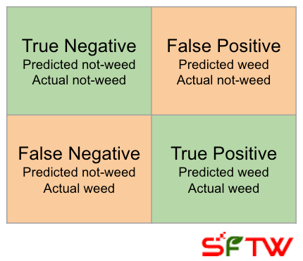
For the case of identification of weeds using a machine learning model, one can construct a simple 2 x 2 matrix.

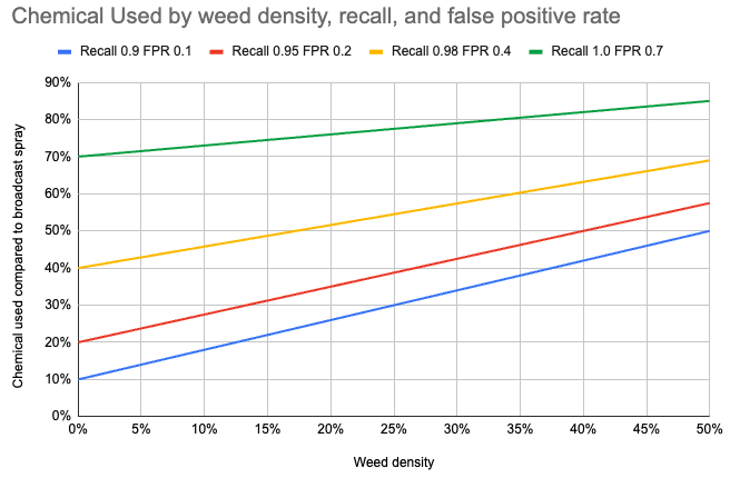
I had presented a simple formula for chemical sprayed in the field as the following,
Chemical sprayed = Weed density x recall + (1 - weed density) x false positive rate.
First term: Weed density is the true number of weeds in the field, and recall indicates what percentage of actual weeds were identified by the model. The model will recommend to spray for weed density times recall rate.
Second term: False positive rate indicates when the model recommends to spray even though it is not a weed. The model will recommend to spray the false positive rate times proportion of the field with no weeds (or 1 - weed density).
Based on this formula, you can calculate the amount of chemical sprayed for different recall, false positive, and weed density rates.
There is an implicit assumption in these calculations. It assumes that the spraying process is executed perfectly at a plant by plant and weed by weed level. This sounds great in theory, but it does not work in practice. In edition 69. The Unbundling of Humans (in agriculture), I had quoted the view of noted geopolitical strategist Peter Zeihan,
Peter Zeihan provides one view for the US Midwest. He imagines a future in which automated equipment with cameras will take photos of each individual plant. The equipment will identify if the plant is a weed, or a crop and assess the health of the crop. It will give it a little jolt of whatever is appropriate (herbicide, pesticide, fertilizer, water etc.). He believes we are on the verge of production increasing by a factor of 2-3 (“on the verge of” is subjective, though within the realm of possibility.) It will turn conventional farming into conventional gardening, with a lower pollution rating and a far lower carbon footprint. (Highlighted by me)
The reality is a bit different.
Given the structure of today’s spraying equipment, there are a certain set of nozzles, set at a certain distance from each other. The nozzles can spray in a particular pattern. Due to this, and other factors like ground speed, spray pressure, and boom height, the spray is done in an area much larger than just a weed (or a plant).
You can get a sense of what it means, and what is its impact on actual savings by looking at the footnotes of John Deere’s, See & Spray Select product page. The product page indicates savings of 77% under certain conditions.
Based on tank-level sensor values taken at a steady state on John Deere sprayers equipped with and without See & Spray™ Select, before and after covering 75,000 acres of fallow ground with a typical weed pressure of 3,000 weeds per acre, using small and medium spray-length settings starting at 2.3 to 3.2 ft. (0.7 to 1 m) and average growing conditions (seasonal precipitation and temperature) across the US and Canadian plains and Australian farms. Spray-length settings varied based on ground speed, spray pressure, and boom height. Sprayers were equipped with current hardware and software at time of study. Individual results may vary based on field and growing conditions, weed pressure, spray-length settings, and software version. (Highlights by me)
The footnote talks about the weed pressure (I had called it out as weed density). As I mentioned earlier, the spray is done in an area larger than a single spot. In the case of see & spray select, the length of the spray area is between 70 centimeter, and 1 meter, and it is dependent on the factors mentioned in the footnote.
To understand this better, let us take a look at a hypothetical scenario.
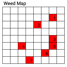
Let us say you have a field with 64 spots (8 x 8) for plants or weeds, and let us assume there are 7 weeds in the field. In the best case scenario, with perfect weed identification and spot spraying, your maximum theoretical chemical savings (compared to 100% broadcast spray) are (64 - 7) / 64 = 89%.
A pogo stick
Now as we discussed last time, due to model performance the reality can be different. Let us assume a less than perfect precision and recall numbers on the model as shown below.
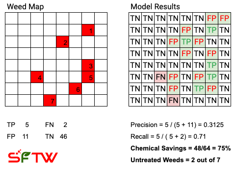
For reference, TP = True Positive (not toilet paper!), FP = False Positive, FN = False Negative, and TN = True Negative.
In this case, we are assuming that the spray can hit each of the squares perfectly. The spray can be likened to the round peg of a pogo stick, which is small and is stamping out any square which has been identified by the model as a weed.
As you can see, in this case the chemical savings are less than the theoretical maximum, and at the same time, it misses 2 out of the 7 weeds (highlighted as FN, False Negative)
Shaq’s sneakers
Now let us assume that the spray area is bigger than the round peg of a pogo-stick. Let us assume it is as big as Shaq’s number 22/23 shoe. Imagine Shaq is stomping on plants, whenever the model thinks there is a weed present in the area which can be stomped by Shaq’s sneakers. In the schematic below, the field is now split into 16 squares, instead of the 64 at the most granular level, and the spraying area minimum is equal to one of the 16 squares. The presence of a weed in a square, should ideally cause the square to be sprayed. Based on these assumptions, a possible scenario with Shaq’s sneakers is as follows:
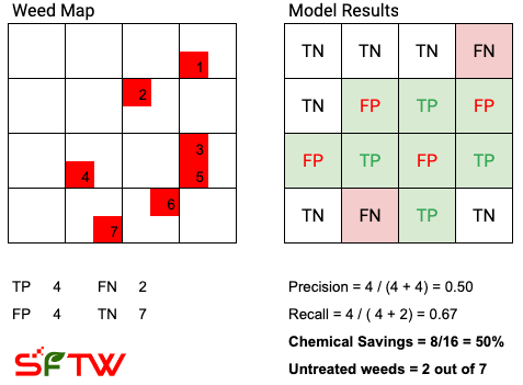
For reference, TP = True Positive, FP = False Positive, FN = False Negative, and TN = True Negative.
The chemical savings drop to 50%, and the number of untreated weeds is still the same due to 2 false negatives. As the spray area increases, you are getting closer to broadcast spray, and your chemical savings will drop.
Snowshoes
What happens when you make the spray area even bigger? What if we divide the field into 4 squares only, instead of 64 squares. It is like wearing those snowshoes made from old tennis rackets.
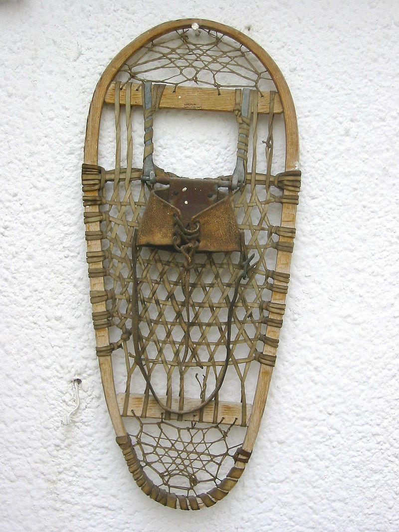
Snowshoe image from Wikipedia
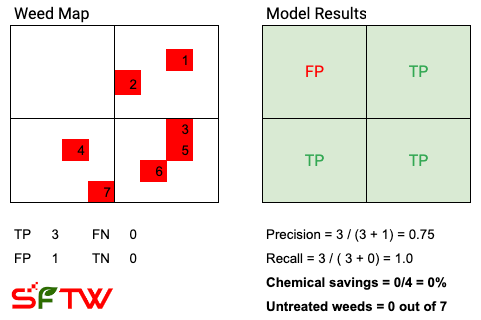
For reference, TP = True Positive, FP = False Positive, FN = False Negative, and TN = True Negative.
In the above example, the model thinks there is a weed in the top left quadrant, and due to this the sprayer sprays the entire top left quadrant. The chemical savings are 0% and the number of untreated weeds is 0. The results in this case are similar to a broadcast spray application.
Chemical savings is not a straightforward metric to calculate. The mechanics of spraying, sprayer design, and the difficulty of spraying each plant individually, forces the sprayer to spray an area which is larger than a plant.
When you see chemical savings as being touted as the main value driver, you should question the provider on topics like precision and recall (discussed in edition 138), speed (discussed in edition 139), spray length size (discussed this week in edition 140). There are other parameters which have an impact on the actual chemical savings, but the issues discussed in 138 through 140 are the most important.
The most important takeaway from this analysis is that footnotes are where the fun is!
